The bigger picture in 2013

Regular readers of this blog know that I love to show off the neat things you can do with IDL, usually with some code. I thought I’d try something different today, though. As product manager, I help set the agenda for IDL development. So, here’s a look at where we’re going with IDL in the near future.

The big themes for IDL in 2013 are:

• visualization
• file access

In the IDL releases this year (8.2.2 in February, 8.2.3 in May and 8.3 this fall), we’re trying to tie development (including improvements, new features and bugfixes) to these themes. Outside issues arise and are addressed, but we’re trying to prioritize stories that fit these themes. So far, this has included new (New) Graphics routines like SCATTERPLOT, BOXPLOT, and soon, BUBBLEPLOT and VOLUME, as well as continued improvements to the performance and usability of NG. For file access, we’ve updated our HDF4, HDF-EOS and CDF libraries, and updates to netCDF, HDF5 and GRIB are on the way.

Looking at the 2013 releases as a whole, I think we’re making good progress in addressing these themes.

(If I get egged on enough, I’ll talk about what we’re thinking about for IDL in 2014, too.)

Coming soon: IDL 8.2.3

IDL 8.2.3 is scheduled to be released on May 21. While this is primarily a maintenance release, we’ve included several new routines. They are:

• BUBBLEPLOT
• VOLUME
• FILE_ZIP
• FILE_UNZIP
• FILE_GZIP
• FILE_GUNZIP
• FILE_TAR
• FILE_UNTAR
• ZLIB_COMPRESS
• ZLIB_UNCOMPRESS
• IDLffVideoRead class
• QUERY_VIDEO
• READ_VIDEO
• WRITE_VIDEO
• TERMINAL_SIZE

BUBBLEPLOT has been an early favorite around VIS. Here’s a sample from Eddie Haskell, the developer who wrote it (click to embiggen):

I’ll post more information on these routines, as well as the rest of what’s included in 8.2.3, on the release date.

Modifying the size and position of a plot

In IDL 8 (a.k.a. New) Graphics, you can interactively move and resize plots in a window. For example, make a test plot in red:

IDL> p = plot([0,1], 'r')

Select the plot by clicking the mouse in the interior of the plot frame. To move the plot, click the frame and drag it. To resize the plot, click and drag a manipulator on the corner or middle of the frame.

Once you’ve moved and/or resized a plot, you can programmatically retrieve its new location and size from the POSITION property. For example, I moved and resized my plot to give:

IDL> print, p.position
      0.12656254      0.47788962      0.54761025      0.88085938

Note that these values are in normalized coordinates (x and y range over a unit interval); the first two values give the (x,y) coordinate of the lower left corner of the plot frame, while the last two values give the coordinate of the upper right corner of the plot frame.

In IDL 8.2.2, we modified the POSITION property so that you can also programmatically set the size and position of a plot; e.g.:

IDL> p.position = [0.50, 0.45, 0.90, 0.90]

The result is a plot in the upper left corner of the window:

A column sort routine

In spreadsheet programs like Excel or LibreOffice, you can apply a sort on a column to every other column in the spreadsheet. IDL’s SORT function doesn’t provide this functionality, but with a little code, we can make it so. The function COLSORT (get the source code here) accepts a 2D array and the zero-based index of the column to sort on. By default, values are sorted in ascending order; a keyword can be set to sort in descending order. Here’s an example of how the routine works.

Start with a 4 x 5 array of numbers:

IDL> a = round(randomu(seed, 4, 5) * 20.0)
IDL> print, 'Original array:', a, format='(a,/,4(i))'
Original array:
           8           6          14          10
           4           9          18           5
           1          11          13          18
           8           9          11           9
           3          19           4          16

Use COLSORT to perform a reverse sort on column index 1 (the second column) and extend the sort to the other columns in the array:

IDL> sort_index = 1
IDL> b = colsort(a, sort_index, /reverse_sort)

Check the result:

IDL> print, 'Sorted (descending) array:', b, format='(a,/,4(i))'
Sorted (descending) array:
           3          19           4          16
           1          11          13          18
           8           9          11           9
           4           9          18           5
           8           6          14          10

This program could be extended to apply to rows and to arrays of higher dimensionality.

Locating NaN and Inf values in an array

(This week’s post is brief because I’m out learning a lot at the 2013 NOAA Satellite Conference!)

The ubiquitous WHERE function can be used to quickly locate values in an array. However, you can’t directly search for the location of IEEE NaN (not a number) and Inf (infinity) values; to do so, you need the FINITE function. Here’s an example.

Start with a simple array:

IDL> a = findgen(5, 2)
IDL> print, a
     0.000000      1.00000      2.00000      3.00000      4.00000
      5.00000      6.00000      7.00000      8.00000      9.00000

and add NaN values at up to three random locations:

IDL> i = floor(randomu(seed, 3)*n_elements(a))
IDL> a[i] = !values.f_nan
IDL> print, a
     0.000000      1.00000      2.00000      3.00000          NaN
          NaN      6.00000      7.00000          NaN      9.00000

OK, so where are the NaNs located? By eye, I can see where they are (indices 4, 5 and 8), but to identify them programmatically, use WHERE with FINITE and “~”, the logical not operator:

IDL> i_nan = where(~finite(a), /null)
IDL> print, i_nan
           4           5           8

Check!

2013 NOAA Satellite Conference

My colleague Thomas Harris (@t_harris) and I will be at the 2013 NOAA Satellite Conference in College Park, MD, next week. We each have a poster:

• T-9: A Rapid Cloud Mask Algorithm  for Suomi NPP VIIRS Imagery EDRs (Piper) [PDF, 2.5 MB]
• W-37: ENVI Services Engine: Earth and Planetary Image Processing for the Cloud (Harris)

If you’re attending this conference, please visit our posters and say hello!

An update to the CURRENT keyword

(Note: I’m out of town this week; this is a short post I banked earlier in the year.)

The IDL 8 (a.k.a. New) Graphics CURRENT keyword got a useful update in IDL 8.2.2: instead of being a Boolean, it now accepts a window reference, which allows me to place a plot in a specific window. For example, if I make two empty windows, W1 and W2:

w1 = window(window_title='Window #1')
w2 = window(window_title='Window #2')

and I want to ensure that a new plot goes into the first window, W1, I can set the CURRENT keyword like so:

p = plot(/test, current=w1, title='I''d like this to be in Window #1')

Check!

Prior to IDL 8.2.2, the SetCurrent method would also do the trick, but I think this syntax is nicer.

Stern Special

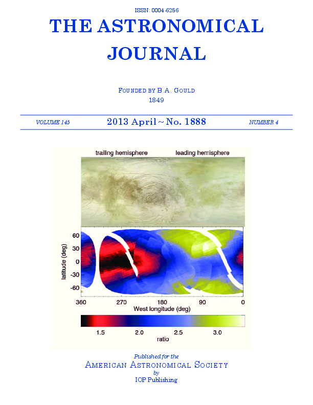
A visualization from an article by the famous (infamous?!) Prof. Mike Brown of Caltech (@plutokiller) is featured on the cover of a recent issue of The Astronomical Journal:

That’s IDL color table 15, Stern Special.

Solar wind visualization at NOAA SWPC

George Millward and his colleagues at the NOAA Space Weather Prediction Center (SWPC) use IDL, among other tools, to study, monitor and forecast solar events that impact GPS, power grids and communications networks on Earth. On the WSA-Enlil Solar Wind Prediction page, Dr. Millward uses IDL Object Graphics to visualize output from a model of solar activity and Javascript to animate the result as a time series. Here’s a sample frame from the animation:

(Click to embiggen.)

From the WSA-Enlil Solar Wind Prediction page, a description of this plot:

The top row plots show predictions of the solar wind density. The bottom row plots show solar wind velocity. The circular plots on the left are a view from above the North Pole of the Sun and Earth, as if looking down from above. The Sun is the yellow dot in the center and the Earth is the green dot on the right. Also shown are the locations of the two STEREO satellites. These plots often depict spiral structures, due to solar rotation. The wedge-shaped plots in the center provide a side view, with north at the top and south at the bottom. The graphs on the right show the model predictions for the time evolution of density and velocity at the locations of Earth and of the two STEREO spacecraft. The yellow vertical line is in sync with the movies on the left, so it is possible to see how values of density and velocity correspond to particular solar wind structures.

Thanks, George! (Are we getting hit by a solar storm at 6 pm today?)

If you’ve done something cool with IDL that you’d like to share, please let me know!

Note: Dr. Millward’s article was also highlighted recently in the “Research Spotlight” section of Eos, Vol. 94, No. 17, 23 April 2013.

VISualize 2013

VISualize is the annual spring IDL and ENVI user group meeting organized by VIS in Washington, DC, and graciously hosted by the World Wildlife Fund at their headquarters. This year, the meeting will take place Tuesday and Wednesday, June 11-12, at the WWF headquarters [map]. The theme for VISualize 2013 is Climate Change and Environmental Monitoring. The registration and call for abstracts is posted online here. If you’re in the area, please register and plan to attend!